Background
The equilibrium shape of a capillary surface such as a liquid meniscus confined within a tube is governed by the Young–Laplace equation, which balances interfacial curvature against hydrostatic pressure:
\begin{equation*}
\nabla \cdot \Bigl( \frac{\nabla u}{\sqrt{1 + |\nabla u|^2}} \Bigr) = Bo\,u + \lambda \quad \text{in } \Omega,
\end{equation*}
where $u(x,y)$ describes the interface height over a cross sectional domain $\Omega \subset \mathbb{R}^2$, $Bo$ is the Bond number, and $\lambda$ is a constant related to the hydrostatic baseline, determined by the fixed liquid volume
\begin{equation*}
V_0 = \iint_{\Omega} u \,dxdy.
\end{equation*}
At the solid boundary, wetting behavior is imposed via Young’s contact angle condition:
\begin{equation*}
\mathbf{n} \cdot \left( \dfrac{\nabla u}{\sqrt{1 + |\nabla u|^2}} \right) = \cos(\theta) \quad \text{on } \partial\Omega.
\end{equation*}
Knowledge about the capillary surface can help in computing evaporation rates or fluid flow in injection systems.
Goal
The objective is to build a PINN that solves the Young–Laplace equation for a fixed cross-section across a range of contact angles $\theta \in [10^\circ,\, 170^\circ]$. In this example we will:
- Implement a PINN with inputs $(x, y, \theta)$ and outputs the water height $u$
- Include the Lagrange multiplier $\lambda(\theta)$ as a learned function
- Compare the results with some reference solution (obtained from the FEM), both in accurarcy and inference speed
Implementation in TorchPhysics
The following implementation can also be found online as a Jupyter Notebook (see here)
First we define variables and parameters that describe the given capillary:
# geometry information
d = 1 # diameter in mm
R = d/2/1e3 # radius in m
norm = R
# surface tension coefficient
sigma = 0.072
# densities (liquid/gas)
rho_l = 998.2
rho_g = 1.225
# gravitational acceleration
g = 9.81
# Bond number
Bo = rho_l*g*R**2/sigma
# calculate normalized cross-sectional area and initial volume
N_points_PDE = 10000
N_points_BC = 5000
A = np.pi*R**2/norm**2
V0 = A*h_l/norm
dA = A/N_points_PDE
dV = V0/N_points_PDE
Now we define all input and output spaces occuring in out problem. Note, that $\theta$ as well as $\lambda$ act as an input (or output) in our problem and are not fixed. Hence, they require an additional space. Followed by the domain, in our case a simple circle for $\Omega$ and an interval for the contact angles $\theta$.
import torchphysics as tp
import numpy as np
X = tp.spaces.R2(variable_name='x')
U = tp.spaces.R1('u')
LAMB = tp.spaces.R1('lamb')
Theta = tp.spaces.R1("theta")

Omega = tp.domains.Circle(space=X, center=[0, 0], radius=1)
interval_theta = tp.domains.Interval(Theta, 10 * np.pi / 180.0, 170 * np.pi / 180.0)
Now we define our neural networks, that we want to train. There are two neural networks to approximate $u$ and $\lambda$ respectively. For this application, we use two simple fully connected networks and combine them in order to send both models to the PDE condition in parallel.
model = tp.models.FCN(input_space=X*Theta, output_space=U,
                      hidden = (50, 50, 50, 50, 50, 50))
model_lamb = tp.models.FCN(input_space=Theta, output_space=LAMB,
                           hidden = (20, 20, 20, 20))

combi_model = tp.models.Parallel(model, model_lamb)
The goal is to find a neural network $u^*: {\Omega}\times\Theta \to \mathbb{R}$ and $\lambda^*: \Theta \to \mathbb{R}$, which approximately satisfies both conditions of the PDE problem above.
The next step is the definition of the training conditions. Here we transform our PDE into some residuals that we minimize in the training. The residuals are denoted by:
- Residual of PDE condition
$$R_{PDE}(u^*, \lambda^*, x, \theta) := \nabla^*\cdot\frac{\nabla^*u^*(x, \theta)}{\sqrt{1+\nabla^*u^*(x, \theta)}^2}-Bo\,u^*(x, \theta)-\lambda^*(\theta) $$ - Residual of Neumann boundary condition
$$R_{BC}(u^*, x, \theta) := \mathbf{n}\cdot\frac{\nabla^*u^*(x, \theta)}{\sqrt{1+\nabla^*u^*(x, \theta)}^2}-\cos(\theta)$$ - Volume constraint (using a discrete approximation of the integral)
$$R_{VOL}(u^*, x^*, \theta^*) := \sum u^*(x^*, \theta^*) \cdot dA - V_0$$
def length_of_grad(grad_u):
    return torch.sqrt(1 + grad_u[:, :1]**2 + grad_u[:, 1:]**2)

def residual_pde_condition(u, x, lamb):
    grad_u = tp.utils.grad(u, x)
    len_grad = length_of_grad(grad_u)
    return tp.utils.div(grad_u/len_grad, x) - Bo*u - lamb

def residual_boundary_condition(u, x, theta):
    grad_u = tp.utils.grad(u, x)
    len_grad = length_of_grad(grad_u)
    normal_vectors = Omega.boundary.normal(x)
    normal_grad = torch.sum(normal_vectors*grad_u, dim=1, keepdim=True)
    return normal_grad/len_grad - torch.cos(theta)

def residual_volume_condition(u):
    return torch.sum(u*dA, dim=0, keepdim=True) - V0
Lastly, we collect these constructions for each condition in an object of the TorchPhysics Condition class which automatically contains the information that the residuals should be minimized in the squared $l_2$-norm. Then we start the training.
pde_condition = PINNCondition(module=combi_model, sampler=sampler_pde_condition, residual_fn=residual_pde_condition)
boundary_condition = PINNCondition(module=model, sampler=sampler_boundary_condition, residual_fn=residual_boundary_condition)
volume_condition = PINNCondition(module=model, sampler=sampler_pde_condition, residual_fn=residual_volume_condition)

training_conditions = [volume_condition, pde_condition, boundary_condition]
optim = tp.OptimizerSetting(optimizer_class=torch.optim.Adam, lr=0.001)
solver = tp.solver.Solver(train_conditions=training_conditions, optimizer_setting=optim)

trainer = pl.Trainer(
    devices=1,
    max_steps=80000,
    logger=False,
    benchmark=True,
    accelerator="gpu",
)
trainer.fit(solver) # start training

Results
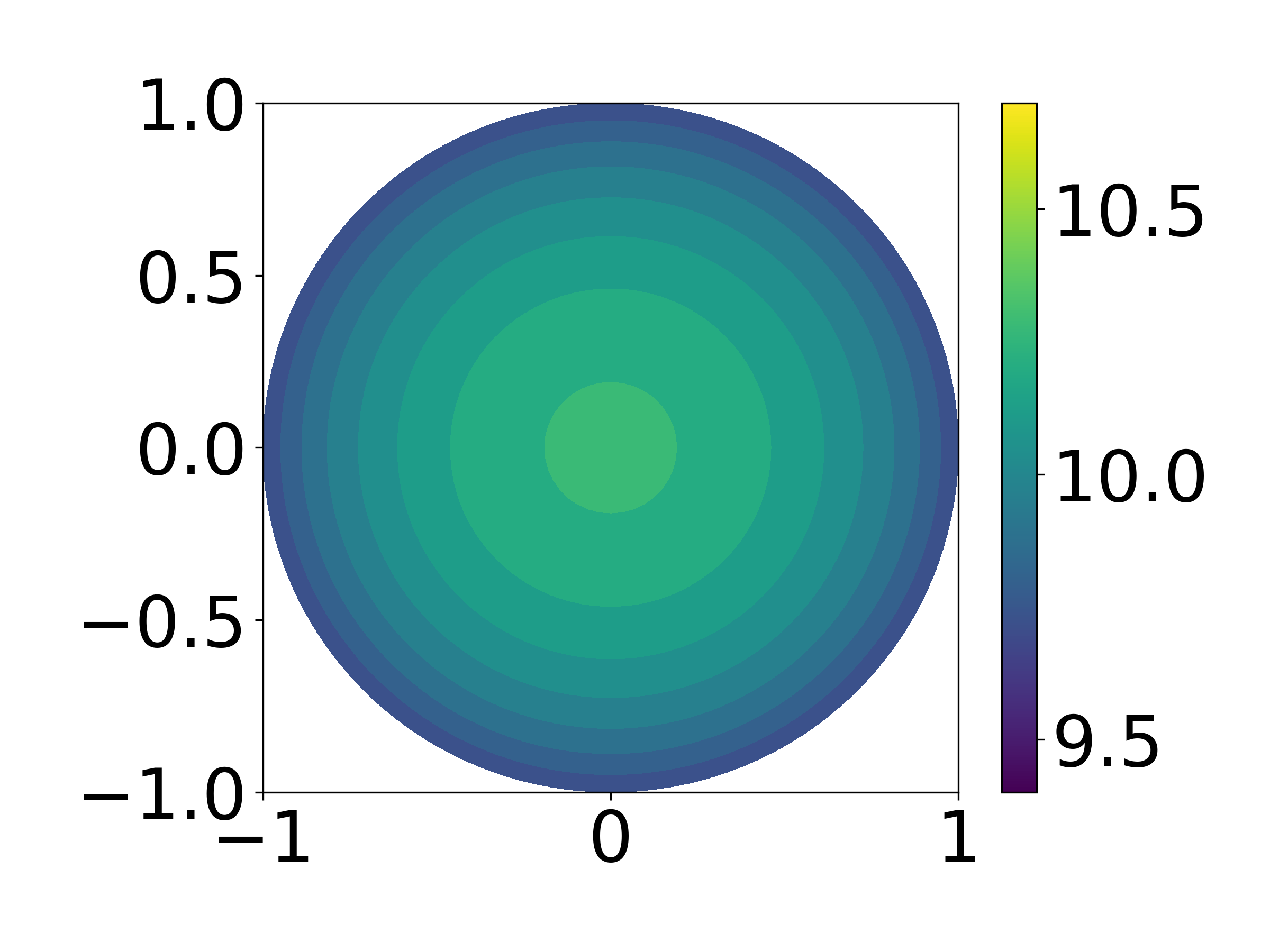
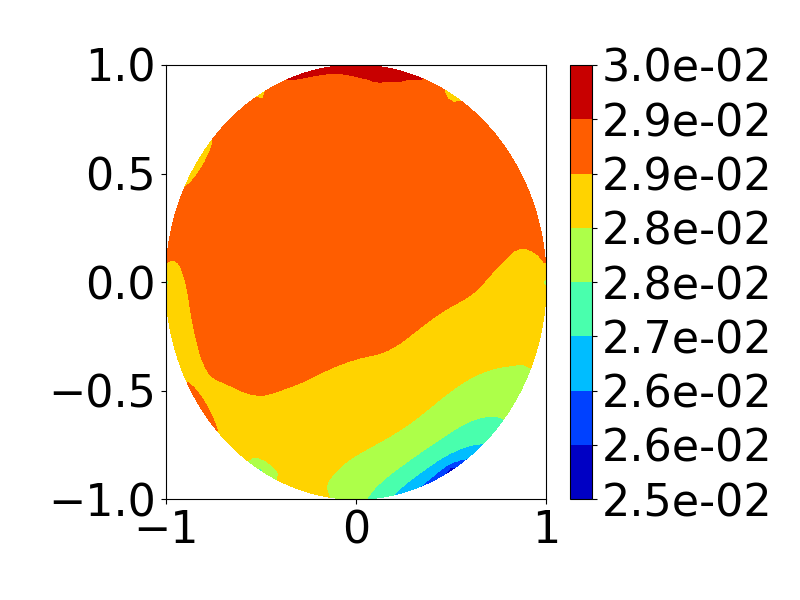
First, we present the solution for a fixed contact angle $\theta = 150^\circ$ in the following images. We achieve an accuracy of around 0.3%.
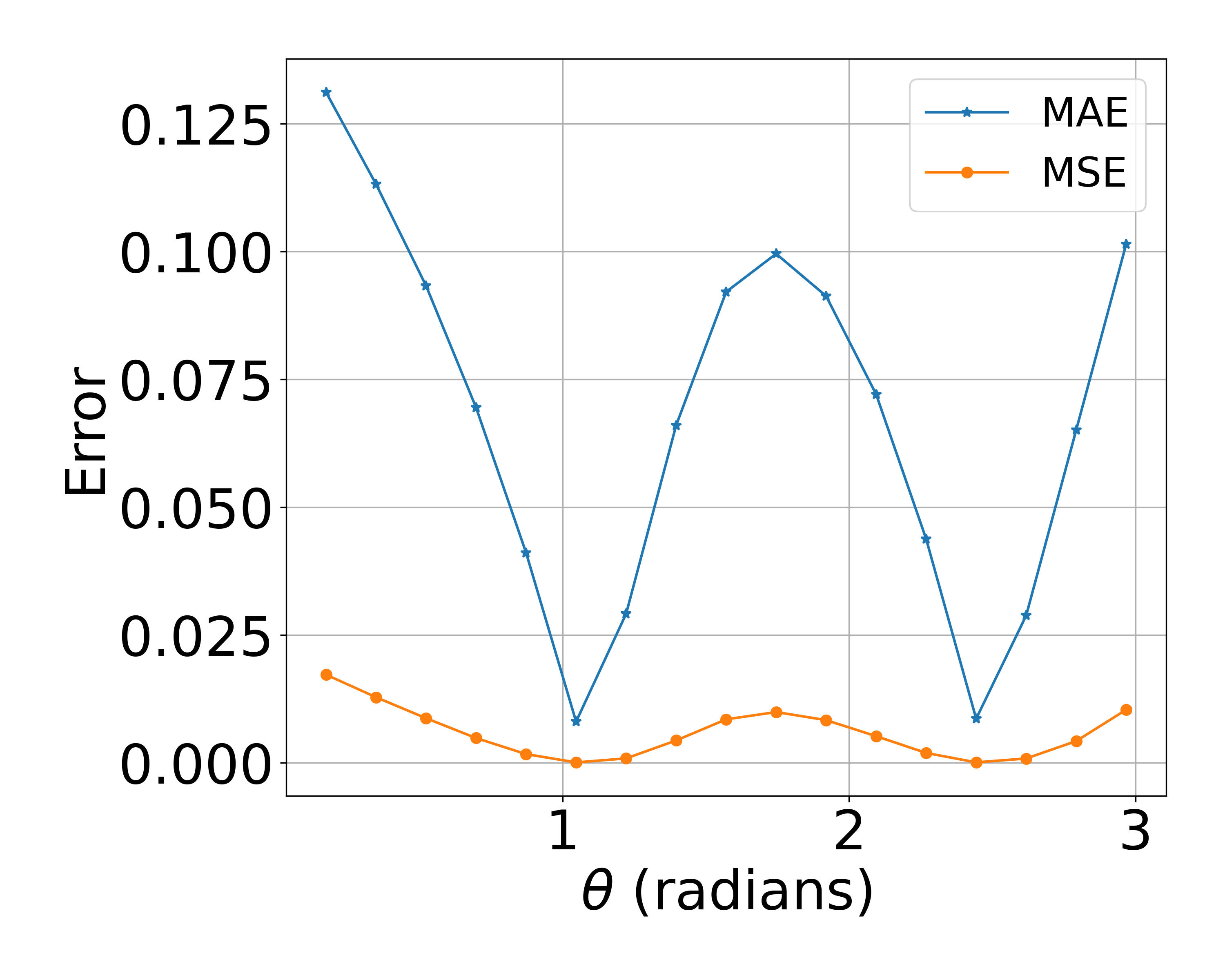
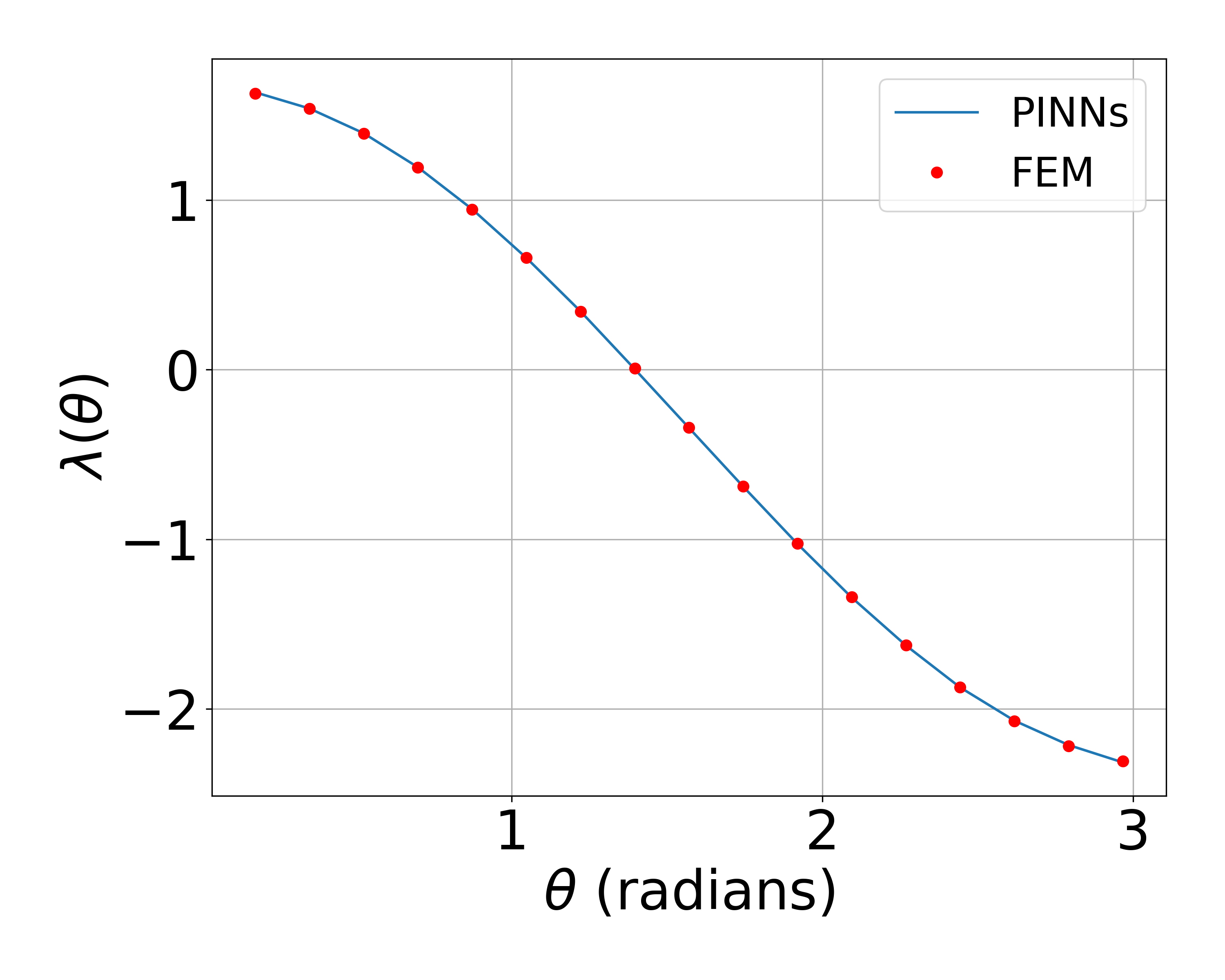
The next two images visualize the error between the PINN solution and FEM solution (both the mean squarred and mean absolute error), as well as the accurarcy of the perdiction of the $\lambda(\theta)$.
Computation Time Comparison
| Method | FEM | PINN on a GPU | PINN on a CPU |
| Training Time | - | 1 h | 4.5 h |
| Inference Time for one $\theta$ | 0.14 s | 0.00092 s | 1.1 s |
| Inference Time for 17 different $\theta$ | 2.4 s | 0.0012 s | 1.4 s |

